앞서 Radiomics에서 많이 사용되고 있는 Feature selection 방법에 대해서 이야기 하였다. 이번에는 조금 더 세분화하여 설명해보도록 하겠다.
14 feature selection methods & 12 classification methods in terms of predictive performance and stability.
Methods
❗ Radiomic Features
A total of 440 radiomic features were used and divided into 4 feature groups.
1) tumor intensity
- intensity of histogram
2) shape
- 3D geometric properties of the tumor
3) texture
- GLCM: gray level co-occurrence matrices
- GLRLM: gray level run length matrices
⇨ quantified the intra-tumor heterogeneity
4) wavelet features
- transformed domain representations of the intensity and textural features.
❗ Datasets
• survival time > 2 years ⇨ 1
• survival time < 2 years ⇨ 0
- 310 lung cancer patients in training cohort, and 154 patients in validation cohort.
- All features were normalised using Z-score normalisation.
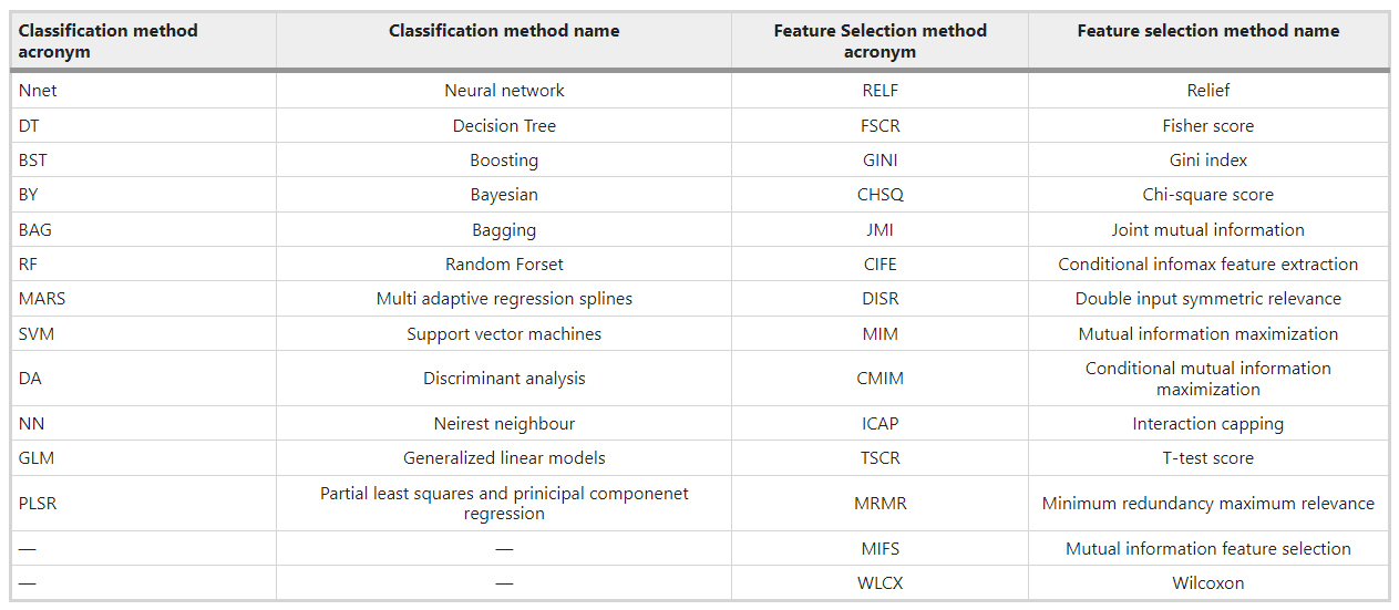
❗ Feature Selection Methods
- 14 feature selection methods based on filter approaches were used.
- 선정기준: simplicity, computational efficiency, popularity in literature
- Fisher score
- Relief
- T-score
- Chi-square
- Wilcoxon
- Gini index
- Mutual information maximisation
- Mutual information feature selection
- Minimum redundancy maximum relevance
- Conditional informax feature extraction
- Joint mutual information
- Conditional mutual information maximisation
- Interaction capping
- Double input symmetric relevance
❗ Classifiers
- 12 machine learning based classification methods were considered.
- supervised learning task로 training set, validation set으로 나눔
- 10 fold cross validation was used
- predictive performance evaluation: AUC
- Bagging
- Bayesian
- Boosting
- Decision trees
- Discriminant analysis
- Generalised linear models
- Multiple adaptive regression splines
- Nearest neighbours
- Neural networks
- Partial least square and principle component regression
- Random forests
- Support vector machines
Analysis
Predictive Performance of Feature Selection Methods
- feature의 개수를 (n = 5, 10, 15, 20, ..., 50) 점차 늘려가며 AUC 값들의 중앙값 계산
Results
a total of 440 radiomic features were extracted from the segmented tumor regions
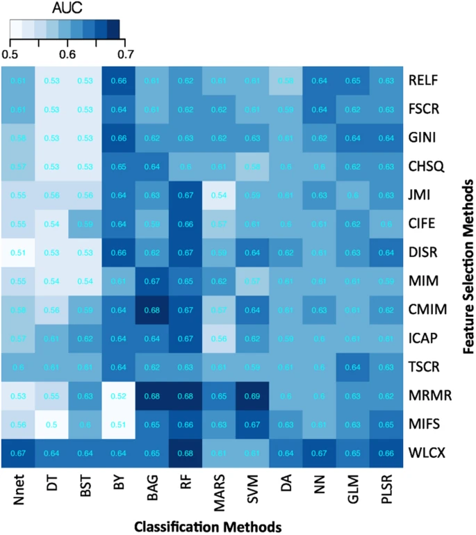
Predictive performance of feature selection and classification methods
• AUC was used for assessing predictive performance of different feature selection and classification methods.
✅ Classification
👍 Random Forest showed the highest predictive performance as a classifier.
(AUC = 0.66 ± 0.03)
👎 Decision Tree had the lowest predictive performance.
(AUC = 0.54 ± 0.04)
✅ Feature selection
👍 Wilcoxon test based methods showed the highest predictive performance
(AUC = 0.65 ± 0.02)
👎 Chi-square & Conditional informax feature extraction displayed the lowest predictive performance. (AUC = 0.60 ± 0.03)
Stability of the feature selection and classification methods
✅ Feature selection
👍 Mutual Information Maximisation was the most stable (stability = 0.94 ± 0.02)
👍 Relief was the second best (stability = 0.91 ± 0.05)
👎 GINI(GINI index), JMI(Joint mutual information), CHSQ(Chi-square), DISR(Double input symmetric relevance), CIFE(Conditional informax feature extraction) showed relatively low stability.
✅ Classification
- RSD(Relative standard deviation) were used for measuring empirical stability.
👍 Bayesian classifier was the best (RSD = 0.86%)
👍 Generalised linear models was the second best (RSD = 2.19%)
👍 Partial least square and principle component regression was the third best (RSD = 2.24%)
👎 Boosting had the lowest stability among the classification methods.
Stability and Predictive Performance
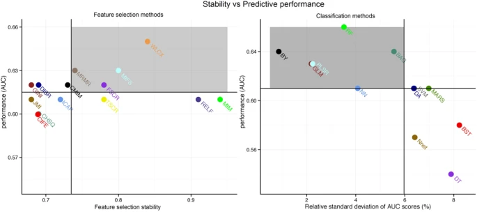
✅ 👍 Feature selection methods
Wilcoxon (stability = 0.84 ± 0.05, AUC = 0.65 ± 0.02)
Mutual information feature selection (stability = 0.8 ± 0.03, AUC = 0.63 ± 0.03)
Minimum redundancy maximum relevance (stability = 0.74 ± 0.03, AUC = 0.63 ± 0.03)
Fisher score (stability = 0.78 ± 0.08, AUC = 0.62 ± 0.04)
are preferred as their stability and predictive performance was higher than corresponding median values(stability=0.735, AUC=0.615) across all feature selection methods.
✅ 👍 Classification methods
RF (RSD = 3.52%, AUC = 0.66 ± 0.03)
BY (RSD = 0.86%, AUC = 0.64 ± 0.05)
BAG (RSD = 5.56%, AUC = 0.64 ± 0.03)
GLM (RSD = 2.19%, AUC = 0.63 ± 0.02)
PLSR (RSD = 2.24%, AUC = 0.63 ± 0.02)
showed that the stability and predictive performance was higher than the corresponding median values(RSD = 5.93%, AUC = 0.61).
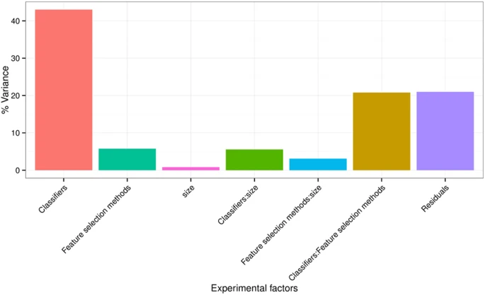
Experimental Factors Affecting the Radiomics Based Survival Prediction
- 3 experimental factors (feature selection methods, classification methods, and the number of selected features) 의 effect를 quantify하기 위해 AUC score에 대한 ANOVA 실시
- ANOVA result: all 3 factors and their interactions are significant.
- Classification method was the most dominant source of variability (34.21%)
- Feature selection accounted for 6.25%
- Classification X Feature selection interaction explained 23.03%
- Size of the selected feature subset only shared 1.65% of the total variance
Discussion
Feature selection methods는 크게 3 카테고리로 나눌 수 있음
(1) filter methods
- This paper only investigated filter methods as these are classifier independent.
• simple feature ranking methods based on some heuristic scoring criterion
• computationally efficient
• high generalisability and scalability
(2) wrapper methods
• classifier dependent
⇨ may produce feature subsets that are overly specific to the classifiers, hence low generalisability
• search through the whole feature space and identify a relevant and non-redundant feature subset.
• computationally expensive
(3) embedded methods
• classifier dependent
⇨ lacks in the generalisability
• incorporate feature selection as a part of training process
• computationally efficient as compared to the wrappers.
Filter Methods
- J : scoring criterion (relevance index)
- Y : class labels
- X : set of all features
- Xk : the feature to be evaluated
- S : the set of already selected features
위 내용을 작성할 때 Parmar, C., Grossmann, P., Bussink, J. et al. Machine Learning methods for Quantitative Radiomic Biomarkers. Sci Rep 5, 13087 (2015). 해당 논문을 참고하였음.
댓글
댓글 쓰기