Statistics: reproducibility, reliability, repeatability in Radiomics 기본 콘텐츠로 건너뛰기

Statistics: reproducibility, reliability, repeatability in Radiomics

Koo, Terry K, and Mae Y Li. “A Guideline of Selecting and Reporting Intraclass Correlation Coefficients for Reliability Research.” Journal of chiropractic medicine vol. 15,2 (2016): 155-63. doi:10.1016/j.jcm.2016.02.012

Taha, Abdel Aziz, and Allan Hanbury. “Metrics for evaluating 3D medical image segmentation: analysis, selection, and tool.” BMC medical imaging vol. 15 29. 12 Aug. 2015, doi:10.1186/s12880-015-0068-x

wikipedia

김장우, and 김종효. "3 차원 의료 영상 분할 평가 지표에 관한 고찰." 대한의학영상정보학회지 23.1 (2017): 14-20.


자동 영상 분할 결과의 유사도를 정량적으로 표현할 때, Dice similarity coefficient를 많이 사용함.


Dice Similarity Coefficient (DSC)는 대표적인 overlap 기반 평가 지표

Intraclass Correlation Coefficients (ICC)는 대표적인 확률 기반 평가 지표


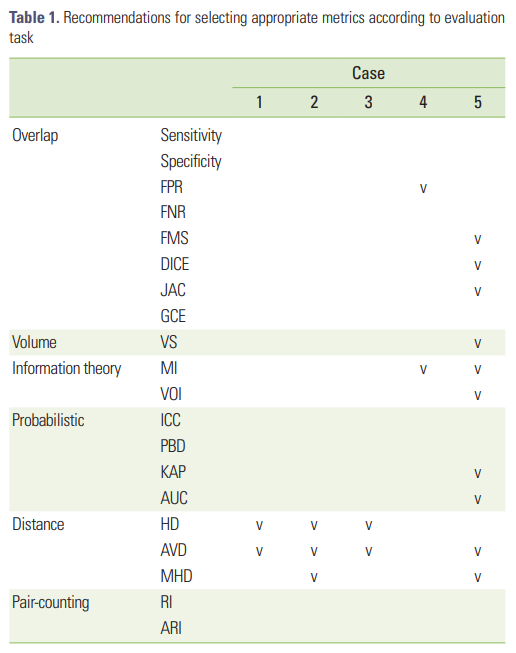
각 케이스에 적용할 수 있는 metrics는 다음 테이블 참조(링크)

Table 1 (Taha, Hanbury 2015)


Difference between DSC and ICC

  • Dice Similarity Coefficient is a measure of how much 2 segmentations overlap in volume. The higher DSC, the better correspondence in volume between 2 raters.
  • ICC measures a correlation between two independent approaches on a series of data


Dice Similarity Coefficient

• DSC = 2|X ⋂ Y| / ( |X| + |Y| )

    X, Y = Given sets

    |X| = cardinalities (집합의 크기) of the set X

    |Y| = cardinalities (집합의 크기) of the set Y

• DSC = 2TP / (2TP+FP+FN)

댓글

이 블로그의 인기 게시물

Radiomics: Feature selection 3

  Demircioğlu, Aydin PhD  Benchmarking Feature Selection Methods in Radiomics, Investigative Radiology: January 18, 2022 - Volume - Issue - doi: 10.1097/RLI.0000000000000855 High dimensionality of the datasets and small sample sizes are critical problems in radiomics. Therefore, removing redundant features and irrelevant features is needed. Overall, per dataset,  30 different feature selection methods + 10 classifiers + 70 hyperparameter settings After each feature selection method, 1, 2, ..., 64 features were selected. Altogether, 14,700=30✕70 ✕7 models were fitted, each with a 10-fold cross-validation . More complex methods are more unstable than simpler feature selection methods. LASSO performed best when analysing the predictive performance , though it showed only average feature stability . Longer training times and higher computational complexity of the feature selection method do not mean for high predictive performance necessarily. Obtaining a more stable mode...

통계 : Dummy Variable Trap

 Regression model을 만들다 보면, 독립변수로 명목형 변수를 사용할 때가 많다. 지역이나 성별, biomaker유/무 등이 대표적으로 많이 사용되는 명목형 변수로, 특히 medical 저널에서는 성별을 covariate으로 취급하여 성별에 따른 종속변수의 차이를 보고자 할 때가 많다. 명목형 변수들은 Dummy Variable로 바꾸어서 regression model을 만드는데, one hot 인코딩 방식으로 더미 변수들을 만든다. 예를 들면,  ❕ male=0, female=1 ❕ Biomarker유=1, Biomarker무=0 이런식으로 만든다. 이와 같은 binary 데이터들은 더미 변수로 만드는 것도 쉽고 큰 문제가 되지 않는다. one-hot encoding의 이유는, 0과 1 대신 빨간색, 녹색, 파란색을 1,2,3 으로 코딩해버리면, 적합한 모델은 숫자가 더 큰 3을 빨간색보다 더 중요한 인자로 생각하게 되기 때문이다. 학력처럼 순서형이면 각 숫자에 의미가 있지만 여러 컬러처럼 단순 명목형일 때에는 one-hot 인코딩을 해야한다.  (단, 컬러가 연함 - 진함과 같이 순서형이라면 굳이 one-hot 인코딩을 안해도 된다.) one-hot encoding 의 예시는 아래 세 가지 카테고리로 보면 더 명확하게 이해가 된다. (image출처: https://towardsdatascience.com/encoding-categorical-variables-one-hot-vs-dummy-encoding-6d5b9c46e2db) 그럼 binary 말고 여러 카테고리가 있는 변수의 경우는 어떤 식으로 더미 변수를 만들까? Regression 모델을 만들 때에는 k개의 카테고리가 있다면, k-1개의 더미변수를 생성하게 된다. 위 그림에서 Blue일 때, d1, d2, d3 모두 0으로 코딩해도 Red, Green과 차이가 있으므로, d1과 d2만 만들어도 무방하다는 의미이다. 즉, d1과 d2가 0일 때, Blue가...

수리통계학 - 이산형 확률변수의 확률분포

 이산형 확률분포의 종류  - 베르누이분포, 이항분포, 이산형균등분포, 기하분포, 초기하분포, 음이항 분포, 포아송 분포 등 이산형 확률변수의 적률생성함수는 다음과 같은 형태로 표현된다. $$ M_{X}(t)=E(e^{tX})=\sum_{x=0}^{\infty}e^{tx}f(x) $$ 1. 베르누이 분포 베르누이 시행의 확률변수 X의 분포는 X=1의 확률에 의해 정의된다. (X=0 or 1) P=P(X=1)=P(성공 ) 베르누이 시행의 확률질량함수 f(x)는 $$ f(x) = p^{x}(1-p)^{1-x}, x=0, 1 $$ 베르누이 분포의 기댓값과 분산은 다음과 같다. E(X)= p , Var(X)= p (1- p ) 베르누이분포의 적률생성함수는 다음과 같다. $$ M(t)=E(e^{tx})=(1-p)+pe^{t} $$ 적률생성함수 유도 과정은 아래와 같이 진행할 수 있다. $$ M(t)=E(e^{tX})=\sum_{x=0}^{1}e^{tx}f(x)=\sum_{x=0}^{1}e^{tx}p^{x}(1-p)^{1-x}=e^{0}p^{0}(1-p)^{1}+e^{t}p^{1}(1-p)^{0}=(1-p)+pe^{t} $$ 적률생성함수를 t에 대해 1차 미분한 후 t값에 0을 대입하면 평균을 도출할 수 있다. 베르누이 분포의 적률생성함수를 1차 미분하면  $$ M(t)=(1-p)+pe^{t}\Rightarrow M^{'}(t)=\frac{d}{dt}(1-p+pe^{t})=pe^{t} \Rightarrow M^{'}(0)=p $$ 2. 이항분포 베르누이 시행을 독립적으로 n번 반복하여 시행한 경우, 성공한 총 횟수를 X라 정의하면, 이 확률변수 X는 이항분포를 따른다. 이항분포의 확률질량함수 f(x)는 다음과 같다. $$ f(x)=\binom{n}{x}p^{x}(1-p)^{n-x}, x= 0,1,2,...,n $$ 이항분포의 기댓값 E(X)= np , Var(X)= np (1- p ) 이다. 이항분포 ...